Key features

The introduction begins with a familiar example. After that we gather main features of the basic user interface. The rest of the features is a collection of different use cases through code examples.

Intuitive interface

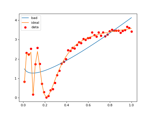
A gammy model can be instantiated “on the fly” by algebraic operations of simpler terms. Below x is a convenience tool (function) for mapping inputs.

import matplotlib.pyplot as plt
import numpy as np

import gammy
from gammy.arraymapper import x
from gammy.models.bayespy import GAM


# Simulate data
input_data = np.linspace(0.01, 1, 50)
y = (
   1.3 + np.sin(1 / input_data) * np.exp(input_data) +
   0.1 * np.random.randn(50)
)

# A totally non-sense model, just an example
bias = gammy.Scalar()
slope = gammy.Scalar()
k = gammy.Scalar()
formula = bias + slope * x + k * x ** (1/2)
model_bad = GAM(formula).fit(input_data, y)

# Ideal model with a user-defined function basis
basis = [
    lambda t: np.sin(1 / t) * np.exp(t),
    lambda t: np.ones(len(t))
]

formula = gammy.Formula(
    terms=[basis],
    # mean and inverse covariance (precision matrix)
    prior=(np.zeros(2), 1e-6 * np.eye(2))
)
model_ideal = GAM(formula).fit(input_data, y)

plt.scatter(input_data, y, c="r", label="data")
plt.plot(input_data, model_bad.predict(input_data), label="bad")
plt.plot(input_data, model_ideal.predict(input_data), label="ideal")
plt.legend()

plt.show()

(Source code)

The basic building block of a Gammy model is a formula object which defines the function basis in terms of which the model is expressed. The package implements a collection of readily usable formulae that can be combined by basic algebraic operations. As seen in, we can define a new formula from existing formulae as follows:

# Formula of a straight line
>>> formula = gammy.Scalar() * x + gammy.Scalar()

The object x is an instance of gammy.ArrayMapper which is a short-hand for defining input data maps as if they were just Numpy arrays.

A formula also holds information of the prior distribution of the implied model coefficients

>>> mean = 0
>>> var = 2
>>> formula = gammy.Scalar((mean, var)) * x + gammy.Scalar((0, 1))
>>> formula.prior
(array([0, 0]), array([[2, 0],
       [0, 1]]))

In higher dimensions we need to use numpy indexing, e.g.:

>>> formula = gammy.Scalar() * x[:, 0] * x[:, 1] + gammy.Scalar()
>>> formula.prior
(array([0, 0]), array([[1.e-06, 0.e+00],
       [0.e+00, 1.e-06]]))

It is easy to define your own formulae:

>>> sine = gammy.Formula([np.sin], (0, 1))
>>> cosine = gammy.Formula([np.cos], (1, 2))
>>> tangent = gammy.Formula([np.tan], (2, 3))
>>> formula = sine + cosine + tangent
>>> formula.prior
(array([0, 1, 2]), array([[1, 0, 0],
       [0, 2, 0],
       [0, 0, 3]]))

Fitting and predicting

The package provides two alternative interfaces for estimating formula coefficients, and subsequently, predicting. The BayesPy based model and the “raw” NumPy based model. The former uses Variational Bayes and the latter basic linear algebra. The BayesPy interface also supports estimating additive noise variance parameter.

>>> formula = gammy.Scalar() * x + gammy.Scalar()
>>> y = np.array([1 + 0, 1 + 1, 1 + 2, 1 + 3])
>>> input_data = np.array([0, 1, 2, 3])
>>> tau = gammy.numpy.Delta(1)  # Noise inverse variance
>>> np_model = gammy.numpy.GAM(formula, tau).fit(input_data, y)
>>> bp_model = gammy.bayespy.GAM(formula).fit(input_data, y)
>>> np_model.mean_theta
[array([1.0000001]), array([0.9999996])]
>>> bp_model.predict(input_data)
array([1., 2., 3., 4.])
>>> (mu, var) = bp_model.predict_variance(input_data)
>>> mu  # Posterior predictive mean
array([1., 2., 3., 4.])
>>> var  # Posterior predictive variance
array([0.00171644, 0.0013108 , 0.0013108 , 0.00171644])

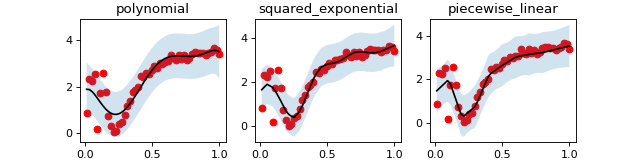
Formula collection

Below are some of the pre-defined constructors that can be used for solving common function estimation problems:

import matplotlib.pyplot as plt
import numpy as np

import gammy
from gammy.arraymapper import x
from gammy.models.bayespy import GAM

# Data
input_data = np.linspace(0.01, 1, 50)
y = (
    1.3 + np.sin(1 / input_data) * np.exp(input_data) +
    0.1 * np.random.randn(50)
)

models = {
    # Polynomial model
    "polynomial": GAM(
        gammy.Polynomial(degrees=range(7))(x)
    ).fit(input_data, y),
    # Smooth Gaussian process model
    "squared_exponential": GAM(
        gammy.Scalar() * x +
        gammy.ExpSquared1d(
            grid=np.arange(0, 1, 0.05),
            corrlen=0.1,
            sigma=2
        )(x)
    ).fit(input_data, y),
    # Piecewise linear model
    "piecewise_linear": GAM(
        gammy.WhiteNoise1d(
            grid=np.arange(0, 1, 0.1),
            sigma=1
        )(x)
    ).fit(input_data, y)
}

# -----------------------------------------
# Posterior predictive confidence intervals
# -----------------------------------------
(fig, axs) = plt.subplots(1, 3, figsize=(8, 2))
for ((name, model), ax) in zip(models.items(), axs):
    # Posterior predictive mean and variance
    (μ, σ) = model.predict_variance(input_data)
    ax.scatter(input_data, y, color="r")
    ax.plot(input_data, model.predict(input_data), color="k")
    ax.fill_between(
        input_data,
        μ - 2 * np.sqrt(σ),
        μ + 2 * np.sqrt(σ),
        alpha=0.2
    )
    ax.set_title(name)

# ---------------------
# Posterior covariances
# ---------------------
(fig, axs) = plt.subplots(1, 3, figsize=(8, 2))
for ((name, model), ax) in zip(models.items(), axs):
    (ax, im) = gammy.plot.covariance_plot(
        model, ax=ax, cmap="rainbow"
    )
    ax.set_title(name)

(Source code)

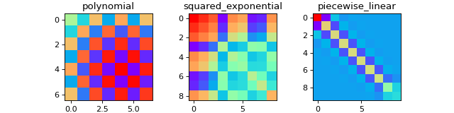
Bayesian statistics

Please read the previous section on how to calculate posterior predictive confidence intervals and posterior/prior covariance information.

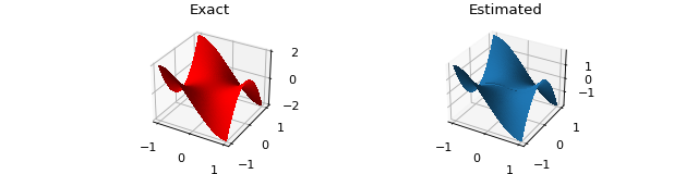
Multivariate terms

It is straightforward to build custom additive model formulas in higher input dimensions using the existing ones. For example, assume that we want to deduce a bivariate function from discrete set of samples:

import matplotlib.pyplot as plt
import numpy as np

import gammy
from gammy.arraymapper import x
from gammy.models.bayespy import GAM

n = 100
input_data = np.vstack(
    [2 * np.random.rand(n) - 1, 2 * np.random.rand(n) - 1]
).T
y = (
    input_data[:, 0] ** 3 -
    3 * input_data[:, 0] * input_data[:, 1] ** 2
)

# The model form can be relaxed with "black box" terms such as
# piecewise linear basis functions:
model = GAM(
    gammy.Polynomial(range(5))(x[:, 0]) +
    gammy.WhiteNoise1d(
        np.arange(-1, 1, 0.05),
        sigma=1
    )(x[:, 1]) * x[:, 0]
).fit(input_data, y)

# Let's check if the model was able to fit correctly:
fig = plt.figure(figsize=(8, 2))
(X, Y) = np.meshgrid(
    np.linspace(-1, 1, 100),
    np.linspace(-1, 1, 100)
)
Z = X ** 3 - 3 * X * Y ** 2
Z_est = model.predict(
    np.hstack([X.reshape(-1, 1), Y.reshape(-1, 1)])
).reshape(100, 100)
ax = fig.add_subplot(121, projection="3d")
ax.set_title("Exact")
ax.plot_surface(
    X, Y, Z, color="r", antialiased=False
)
ax = fig.add_subplot(122, projection="3d")
ax.set_title("Estimated")
ax.plot_surface(
    X, Y, Z_est, antialiased=False
)

(Source code)

Gaussian processes

Theory

In real-world applications usually one doesn’t know closed form expression for the model. One approach in tackling such problems is modeling the unknown function as a Gaussian Process. In practice one tries to estimate the model in the form

\[y = f(x) + \varepsilon, \qquad f(x) \sim \mathcal{N}(\mu, \Sigma_{\rm prior}), \ \ \varepsilon \sim \mathcal{N}(0, \tau^{-1})\]

where \(\varepsilon\) is the additive noise and \(\Sigma_{\rm prior} = K(x, x)\) is a symmetric positive-definite matrix valued function defined by a kernel function \(k(x, x')\):

\[K(x, x) = \left[ k(x_i, x_j) \right]_{i,j=1}^N.\]

The mean and covariance of the Gaussian posterior distribution has closed form:

\[\begin{split}\begin{split} \mu_{\rm post}(x) &= \mu + K(x, x)(K(x, x) + \tau I)^{-1}(y - \mu) \\ \Sigma_{\rm post}(x) &= K(x, x) - K(x, x)(K(x, x) + \tau I)^{-1}K(x, x) \end{split}\end{split}\]

Point estimates such as conditional mean predictions can be easily calculated with the posterior covariance formula.

In Gammy we use a truncated eigendecomposition method which turns the GP regression problem into a basis function regression problem. Let \(A\) be an invertible matrix and consider the change of variables \(w = A(f(x) - \mu)\). Using change of variables for probability densities it is straightforward to deduce that

\[w \sim \mathcal{N}(0, I) \quad {\rm if} \quad A = \Lambda ^{-1/2} U^T\]

where \(U\Lambda U^T\) is the eigendecomposition of \(\Sigma_{\rm prior}\). Note that the eigenvectors (columns of \(U\)) are orthogonal because a covariance matrix is symmetric and positive-definite. Therefore the parameter estimation problem implied by

\[y = \mu + A^{-1} w + \varepsilon= \mu + U \Lambda^{1/2} w + \varepsilon, \quad w \sim \mathcal{N}(0, I), \ \ \varepsilon \sim \mathcal{N}(0, \tau^{-1})\]

is equivalent with the original GP regression problem. In fact, identifying that

\[U\Lambda^{1/2}w = \sum_{n=1}^N w_n\lambda_n(x)^{1/2}u_n(x)\]

we have transformed the original problem into a basis function regression problem where the basis is defined in terms of the (scaled) eigenvectors of the original covariance matrix \(K(x, x)\) evaluated in the grid points.

In Gammy, we use the following algorithm to perform GP regression:

1. Select a fixed grid of evaluation \(x = [x_1, x_2, \ldots, x_N]\)

2. Compute \(U(x)\) and \(\Lambda(x)\) and their linear interpolators.

3. Estimate the weights vector using the Bayesian method \(w\).

4. Evaluate predictions in another grid \(x'\) by interpolation

   \[y_{\rm pred} = \mu + U(x')\Lambda^{1/2}(x')\]

The upside of the used approach are

• Precomputed model for calculating predictions, i.e, for each prediction, we don’t need to solve least squares problem.

• Ability to truncate the covariance if number of data points is large.

Downsides:

• Grid dependence,

• Interpolation errors,

• Doesn’t scale efficiently if the number of input dimensions is large because we use Kronecker product to construct high dimensional bases.

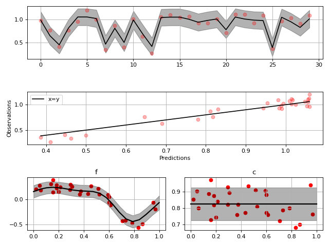
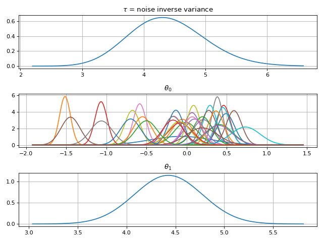
One-dimensional Gaussian Process models

In this example, we have a 1-D noisy dataset \(y\) and the input data are from the interval \([0, 1]\). The model shape is unknown, and is sought in the form

\[y = f(x) + c + \varepsilon\]

where \(f(x)\) is a Gaussian process with a squared exponential prior kernel and \(c\) is an unknown scalar with a normally distributied (wide enough) prior. The additive noise \(\varepsilon\) is normally distributed and zero-mean but it’s variance is estimated from data.

import matplotlib.pyplot as plt
import numpy as np
import pandas as pd

import gammy
from gammy.arraymapper import x


# Simulated dataset
n = 30
input_data = np.random.rand(n)
y = (
   input_data ** 2 * np.sin(2 * np.pi * input_data) + 1 +
   0.1 * np.random.randn(n)  # Simulated pseudo-random noise
)

# Define model
f = gammy.ExpSquared1d(
    grid=np.arange(0, 1, 0.05),
    corrlen=0.1,
    sigma=0.01,
    energy=0.99
)
c = gammy.Scalar()
formula = f(x) + c
model = gammy.models.bayespy.GAM(formula).fit(input_data, y)

#
# Plotting results -----------------------------------------
#

# Plot validation plot
fig1 = gammy.plot.validation_plot(
   model,
   input_data,
   y,
   grid_limits=[0, 1],
   input_maps=[x, x],
   titles=["f", "c"]
)

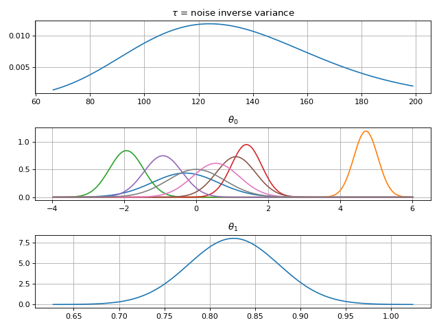
# Parameter posterior density plot
fig2 = gammy.plot.gaussian1d_density_plot(model)

plt.show()

(Source code)

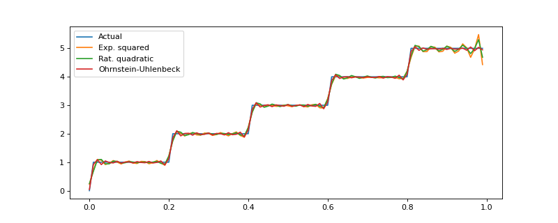
More on Gaussian Process kernels

The GP covariance kernel defines the shape and smoothness of the resulting function estimate. The package implements some of the most typical kernels, and the below example demonstrates how different kernels perform in a hypothetical step function (truncated) estimation problem.

from functools import reduce

import matplotlib.pyplot as plt
import numpy as np

import gammy
from gammy.arraymapper import x


# Define data
input_data = np.arange(0, 1, 0.01)
y = reduce(lambda u, v: u + v, [
    # Staircase function with 5 steps from 0...1
    1.0 * (input_data > c) for c in [0, 0.2, 0.4, 0.6, 0.8]
])

# Kernel parameters
grid = np.arange(0, 1, 0.01)
corrlen = 0.01
sigma = 2

# Define and fit models with different kernels
exp_squared_model = gammy.models.bayespy.GAM(
    gammy.ExpSquared1d(
        grid=grid,
        corrlen=corrlen,
        sigma=sigma,
        energy=0.9
    )(x)
).fit(input_data, y)
rat_quad_model = gammy.models.bayespy.GAM(
    gammy.RationalQuadratic1d(
        grid=grid,
        corrlen=corrlen,
        alpha=1,
        sigma=sigma,
        energy=0.9
    )(x)
).fit(input_data, y)
orn_uhl_model = gammy.models.bayespy.GAM(
    gammy.OrnsteinUhlenbeck1d(
        grid=grid,
        corrlen=corrlen,
        sigma=sigma,
        energy=0.9
    )(x)
).fit(input_data, y)

#
# Plotting results -----------------------------------------
#

ax = plt.figure(figsize=(10, 4)).gca()
ax.plot(input_data, y, label="Actual")
ax.plot(
    input_data,
    exp_squared_model.predict(input_data),
    label="Exp. squared"
)
ax.plot(
    input_data,
    rat_quad_model.predict(input_data),
    label="Rat. quadratic"
)
ax.plot(
    input_data,
    orn_uhl_model.predict(input_data),
    label="Ohrnstein-Uhlenbeck"
)
ax.legend()

(Source code)

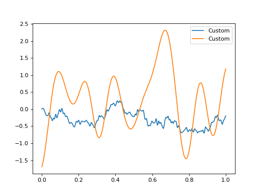
Customize Gaussian Process kernels

It is straightforward to define custom formulas from “positive semidefinite” covariance kernel functions.

import matplotlib.pyplot as plt
import numpy as np

import gammy
from gammy.arraymapper import x


def kernel(x1, x2):
    """Kernel for min(x, x')

    """
    r = lambda t: t.repeat(*t.shape)
    return np.minimum(r(x1), r(x2).T)

def sample(X):
    """Sampling from a GP kernel square-root matrix

    """
    return np.dot(X, np.random.randn(X.shape[1]))

grid = np.arange(0, 1, 0.001)

Minimum = gammy.create_from_kernel1d(kernel)
a = Minimum(grid=grid, energy=0.999)(x)

# Let's compare to exp squared
b = gammy.ExpSquared1d(
    grid=grid,
    corrlen=0.05,
    sigma=1,
    energy=0.999
)(x)

#
# Plotting results -----------------------------------------
#

ax = plt.figure().gca()
ax.plot(grid, sample(a.design_matrix(grid)), label="Custom")
ax.plot(grid, sample(b.design_matrix(grid)), label="Custom")
ax.legend()

plt.show()

(Source code)

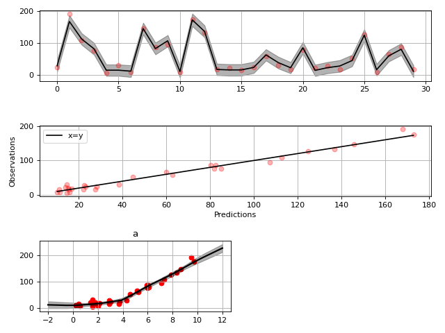
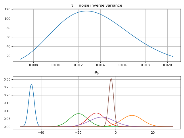
Spline regression

Constructing B-Spline based 1-D basis functions is also supported.

import matplotlib.pyplot as plt
import numpy as np

import gammy
from gammy.arraymapper import x

# Define dummy data
n = 30
input_data = 10 * np.random.rand(n)
y = 2.0 * input_data ** 2 + 7 + 10 * np.random.randn(n)


# Define model
a = gammy.Scalar()

grid = np.arange(0, 11, 2.0)
order = 2
N = len(grid) + order - 2
sigma = 10 ** 2
a = gammy.BSpline1d(
    grid,
    order=order,
    prior=(np.zeros(N), np.identity(N) / sigma),
    extrapolate=True
)
formula = a(x)
model = gammy.models.bayespy.GAM(formula).fit(input_data, y)

#
# Plotting results --------------------------------------------
#

# Plot results
fig = gammy.plot.validation_plot(
    model,
    input_data,
    y,
    grid_limits=[-2, 12],
    input_maps=[x],
    titles=["a"]
)

# Plot parameter probability density functions
fig = gammy.plot.gaussian1d_density_plot(model)

plt.show()

(Source code)

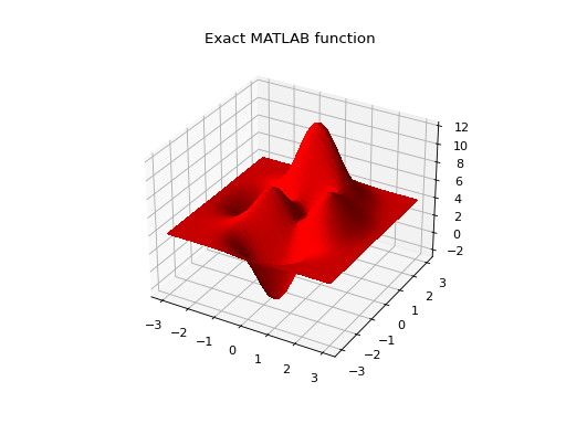
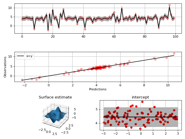
Non-linear manifold regression

In this example we construct a basis corresponding to a multi-variate Gaussian process with a Kronecker structure (see e.g. PyMC3).

Another way to put it, we can form two (or more) -dimensional basis functions given two (or more) one-dimensional formulas. The new combined basis is essentially the outer product of the given bases. The underlying weight prior distribution priors and covariances are constructed using the Kronecker product.

Let create some artificial data using the MATLAB function!

import matplotlib.pyplot as plt
from mpl_toolkits.mplot3d import Axes3D
import numpy as np

import gammy
from gammy.arraymapper import x


# Create some data
n = 100
input_data = np.vstack((
    6 * np.random.rand(n) - 3, 6 * np.random.rand(n) - 3
)).T

def peaks(x, y):
    """The MATLAB function

    """
    return (
        3 * (1 - x) ** 2 * np.exp(-(x ** 2) - (y + 1) ** 2) -
        10 * (x / 5 - x ** 3 - y ** 5) * np.exp(-x ** 2 - y ** 2) -
        1 / 3 * np.exp(-(x + 1) ** 2 - y ** 2)
    )

y = (
    peaks(input_data[:, 0], input_data[:, 1]) + 4 +
    0.3 * np.random.randn(n)
)

# Plot the MATLAB function
X, Y = np.meshgrid(np.linspace(-3, 3, 100), np.linspace(-3, 3, 100))
Z = peaks(X, Y) + 4
ax = plt.figure().add_subplot(111, projection="3d")
ax.plot_surface(X, Y, Z, color="r", antialiased=False)
ax.set_title("Exact MATLAB function")

# Define model
a = gammy.ExpSquared1d(
    np.arange(-3, 3, 0.1),
    corrlen=0.5,
    sigma=4.0,
    energy=0.9
)(x[:, 0])
b = gammy.ExpSquared1d(
    np.arange(-3, 3, 0.1),
    corrlen=0.5,
    sigma=4.0,
    energy=0.9
)(x[:, 1])
A = gammy.Kron(a, b)
bias = gammy.Scalar()
formula = A + bias
model = gammy.models.bayespy.GAM(formula).fit(input_data, y)

#
# Plot results
#

# Validation plot
fig = gammy.plot.validation_plot(
    model,
    input_data,
    y,
    grid_limits=[[-3, 3], [-3, 3]],
    input_maps=[x, x[:, 0]],
    titles=["Surface estimate", "intercept"]
)

# Probability density functions
fig = gammy.plot.gaussian1d_density_plot(model)

(Source code)

Note that same logic could be used to construct higher dimensional bases:

# 3-D formula
formula = gammy.kron(gammy.kron(a, b), c)

and so on.